| 释义 |
Pearson SystemGeneralizes the differential equation for the Gaussian Distribution
 | (1) |
 | (2) |
 , ,  be the roots of be the roots of  . Then the possible types of curves are . Then the possible types of curves are- 0.
 , ,  . E.g., Normal Distribution. . E.g., Normal Distribution. - I.
 , ,  . E.g., Beta Distribution. . E.g., Beta Distribution. - II.
 , ,  , ,  where where  . . - III.
 , ,  , ,  where where  . E.g., Gamma Distribution. This case isintermediate to cases I and VI. . E.g., Gamma Distribution. This case isintermediate to cases I and VI. - IV.
 , ,  . . - V.
 , where , where  . Intermediate to cases IV and VI. . Intermediate to cases IV and VI. - VI.
 , where is the larger root. E.g., Beta Prime Distribution. , where is the larger root. E.g., Beta Prime Distribution. - VII. ,
 , . E.g., Student's t-Distribution. , . E.g., Student's t-Distribution.
Classes IX-XII are discussed in Pearson (1916). See also Craig (in Kenney and Keeping 1951). If a Pearson curve possesses aMode, it will be at  . Let . Let  at and , where these may be at and , where these may be  or or  . If . If also vanishes at , , then the also vanishes at , , then the  th Moment and th Moment and  th Moments exist. th Moments exist. | | | (3) |
giving | |  | (4) |
 | (5) |
 | (6) |
 | (7) |
 , ,
 | (8) |
 | (9) |
 , ,
 | (10) |
 | (11) |
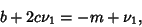
 . Then . Then
Hence  , and , and  so so
 | (15) |
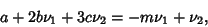
 , ,
 | (16) |
 , ,
 | (17) |
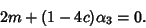
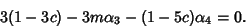
So the parameters  , ,  , and , and  can be written can be written
where
 | (23) |
References
Craig, C. C. ``A New Exposition and Chart for the Pearson System of Frequency Curves.'' Ann. Math. Stat. 7, 16-28, 1936.Kenney, J. F. and Keeping, E. S. Mathematics of Statistics, Pt. 2, 2nd ed. Princeton, NJ: Van Nostrand, p. 107, 1951. Pearson, K. ``Second Supplement to a Memoir on Skew Variation.'' Phil. Trans. A 216, 429-457, 1916.
|

